2. Quickstart
If you have an already installed Python3 environment in your operating system, the easiest way to install Deep-Transit is to using pip:
pip install deep-transit -U
The detailed information can be found in our installation instructions.
Once you have successfully installed the Deep-Transit package, you can download our released model for your transit detection. We have released two pretrained models, one trained from Kepler and the other trained from TESS (download Kepler model, download TESS model).
[1]:
model_path = '/home/ckm/model_Kepler.pth'
After you have downlaod the pretrained model, the transit detection can be fairly easy! For example, we can download a light curve of Kepler-1b with the help of lightkurve.
[2]:
import lightkurve as lk
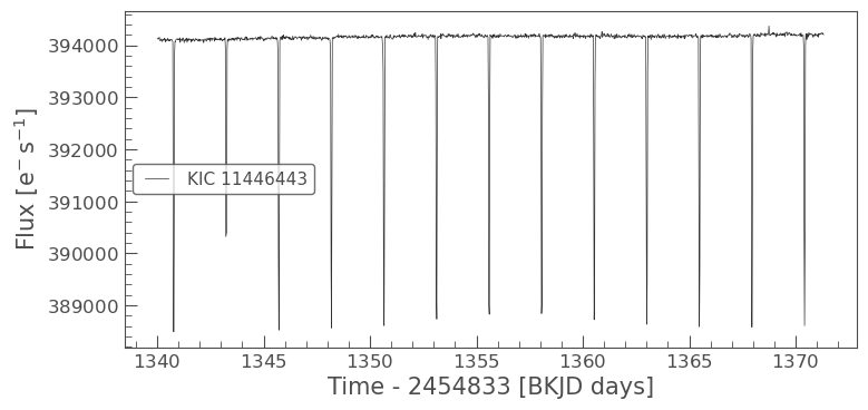
lc = lk.search_lightcurve('Kepler-1b', quarter=14, exptime='long').download();
lc = lc[lc.time.value>1340] # To save computating time
lc.plot()
[2]:
<AxesSubplot:xlabel='Time - 2454833 [BKJD days]', ylabel='Flux [$\\mathrm{e^{-}\\,s^{-1}}$]'>
Our Deep-Transit package can be seamlessly accept a LightCurve object, so the detection can be finished in one line
[3]:
import deep_transit as dt
bboxes = dt.DeepTransit(lc, is_flat=True).transit_detection(model_path)
Loading Model: /home/ckm/model_Kepler.pth
/home/ckm/Deep-Transit/src/deep_transit/dt_lightcurve.py:317: UserWarning: The total number of progress bar is the upper limit.
100%|██████████| 4/4 [00:12<00:00,  3.10s/it]
Now you have finished your first transit detection, you can plot the detected bounding boxes with the light curve.
[4]:
dt.plot_lc_with_bboxes(lc, bboxes, ms=3, marker='o')
[4]:
<AxesSubplot:xlabel='Time (day)', ylabel='Normalized Flux'>
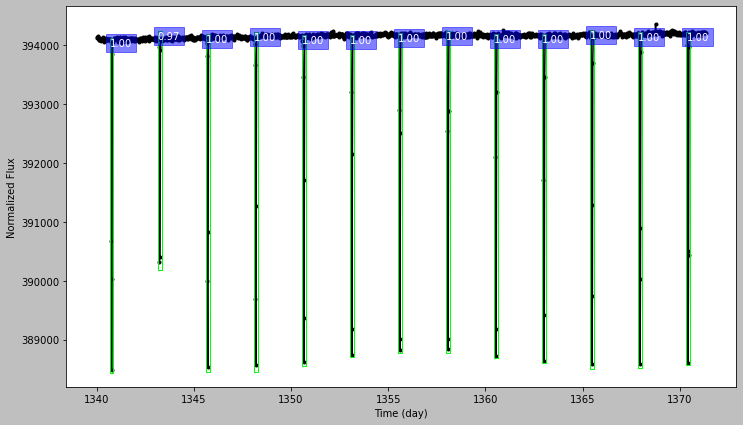
This plot shows the light cuvre with detected transiting signals, the number at the top of each bounding box is the confidence level, which can be an indicator of signal-to-noise ratio.
[ ]: